


Introduction
Profiling all the transcripts expressed in the glomerulus and each renal tubule segment will greatly advance our understanding of the functions and pathophysiology of the kidney. This task requires a precise, unbiased, and high-throughput transcriptomic method that enables researchers to create a catalog┬Āof all the RNA species and accurately measure their quantities in a cell.
However, gene expression profiling methods that have been used in renal transcriptomics such as microarrays [1], [2] or Sanger sequencing of complementary DNAs (cDNAs) [3], [4], [5] suffer from low sensitivity and high false positivity. The utility of microarrays is limited by the requirement of prior knowledge of genes expressed in a cell and by a narrow range of dynamic expression due to signal saturation. Sanger sequencing of cDNAs is low throughput and not sensitive enough to detect lowly expressed transcripts.
RNA sequencing (RNA-seq) uses next-generation sequencing (NGS) technologies to profile the whole transcriptome in a massive┬Āparallel manner [6]. In this method, RNAs of interest [i.e., messenger RNAs (mRNAs), microRNAs, or other noncoding RNAs] are converted into adapter-ligated cDNAs and sequenced in a parallel manner, generating massive amount of short DNA sequences (typically 35ŌĆō100 base pairs) [6]. These nucleotide sequences (commonly called reads) are either mapped to a reference genome or assembled to generate a de novo transcriptome. Reads mapped to the reference genome can be visualized on a genome browser to explore transcriptional activity across the genome or can be counted to quantify the expression level of each transcript. Compared with microarrays or Sanger sequencing, RNA-seq has many advantages, including higher sensitivity (requiring lower amount of RNAs), low false positivity (no background signals originating from cross-hybridization), unlimited range of dynamic expression (no signal saturation), and capability to process many samples in high-throughput settings (many samples can be multiplexed and sequenced in parallel).
Recently, RNA-seq transcriptomic data for glomeruli and 14 different renal tubule segments collected from rat kidneys have been published [7]. This review discusses the technical aspects of RNA-seq profiling of the nephron, focusing on how RNA-seq and classical microdissection can be combined to profile the transcriptomes of the rat nephron. This review does not intend to provide an in-depth review of the NGS technologies. Readers are referred to excellent reviews on the principles of NGS [8], [9]. For more general information on RNA-seq, the author would like to recommend a well-curated online Web site available at http://rnaseq.uoregon.edu/.
Microdissection of renal tubule segments
Collagenase-assisted manual microdissection of renal tubule segments, first reported by Burg et┬Āal┬Āin 1966 [10], has been successfully used in renal physiology for more than 4 decades. This method expanded the scope of renal research to glomeruli and tubule segments that had not been accessible by micropuncture. To collect glomeruli and renal tubule segments for RNA-seq profiling, a protocol previously published in the article by Wright et┬Āal [11] was used with minor modifications. A male Sprague Dawley rat weighing 150ŌĆō200 g is killed by decapitation (Animal Study Protocol No. H-0110R2, approved by the Animal Care and Use Committee, National Heart, Lung, and Blood Institute). After a midline incision of the abdominal wall, the left renal artery is selected by introducing a ligature in the aorta between the left and renal arteries. Then, a thin plastic catheter is introduced through a slit made on the wall of the aorta below the level of the left renal artery, and through this catheter, the left kidney is perfused with 10 mL of ice-cold, bicarbonate-free dissecting solution (NaCl 135┬Āmmol/L; Na2HPO4 1┬Āmmol/L; Na2SO4 1.2┬Āmmol/L; MgSO4 1.2┬Āmmol/L; KCl 5┬Āmmol/L; CaCl2 2┬Āmmol/L; glucose 5.5┬Āmmol/L; and HEPES 5┬Āmmol/L, adjusted to pH 7.4), followed by 10 mL of collagenase solution [1 mg/mL of collagenase B (purified from Clostridium histolyticum, Roche Diagnostics, Indianapolis, IN, USA) and 1 mg/mL of bovine serum albumin (MP Biomedicals, Santa Ana, CA, USA) in the dissecting solution] warmed to 37┬░C. Before use, the dissecting solution in which collagenase and bovine serum albumin are to be dissolved is usually bubbled with 100% O2 for 10 minutes to mitigate hypoxia. It is crucial that the blood in the left kidney is completely removed by the initial perfusion with the dissecting solution┬Ābecause protease inhibitors in the plasma prevent collagenase from acting on the kidney. Although some renal tubule segments (e.g., the cortical collecting duct) can be dissected without collagenase digestion, most parts of the nephron cannot be dissected if the kidney is not properly digested. To facilitate the perfusion process, the wall of the inferior vena cava needs to be cut so that the blood and solution returning from the left kidney via the left renal vein can easily exit the circulation. After the perfusion with the collagenase solution, the left kidney is removed and cut into Ōł╝1 mm3 cubes, put into the same collagenase solution, and incubated in a chamber filled with O2 at 37┬░C for 30ŌĆō90 minutes. The concentration of collagenase and the duration of incubation need to be adjusted, depending on which tissue compartment is going to be dissected. The cortex can be digested in 1% collagenase for 30 minutes. The outer and inner medullas require a higher collagenase concentration and longer duration (1% and 45 minutes for the outer medulla; 3% and up to 90 minutes for the inner medulla), along with hyaluronidase of the same concentration as collagenase. Even with a higher concentration of collagenase, digestion of the inner medulla was successful only once in every 3 or 4 experiments. A thorough pretreatment of the dissecting solution and other apparatuses to inactivate ribonuclease is generally not needed, although general precautions used in RNA works (i.e., wearing gloves, using ribonuclease-inactivating products) need to be followed. This is probably because the content of ribonuclease is not high in the kidney compared with other organs such as the spleen or the pancreas.
After digestion, the tissue chunks are taken out of the collagenase solution, washed twice in ice-cold dissecting solution to end digestion process, and put in a glass dish containing ice-cold dissecting solution. This dish is then brought under a stereomicroscope for microdissection. To minimize tissue degradation, the digested kidney tissue needs to be maintained at a cool temperature, ideally at 4┬░C. It is generally recommended to use a stereomicroscope that has a coolant-circulating system attached to the bottom of the stage of the microscope. If the glass dish containing the digested tissue is maintained at 4┬░C, a microdissection session can be extended up to 4 hours with minimal tissue degradation. For optimal identification of tubule segments, it is better to have the light source for the stereomicroscope below the object stage.
The digested kidney tissue is examined using Dumont No.┬Ā5┬Āforceps (https://www.dumonttweezers.com/Tweezer/Tweezer/469). Before use, the tips of the tweezers need to be sharpened and polished with a piece of sandpaper so that the tweezers can easily grab and manipulate tubule segments and a dissected tubule segment or other irrelevant tissue does not stick to the surface of the tweezer tips. The degree of tissue digestion can be assessed by trying to grab and separate tissue chunk using tweezers. If it is too difficult to separate tubules from surrounding tissue, the tissue chunks can be transferred back to the collagenase solution for more digestion (up to 5ŌĆō10 minutes).
Identifying individual renal tubule segments requires working knowledge of renal anatomy. Through practice, the dissector becomes more and more familiar with the morphology and locations of individual renal tubule segments. The anatomical and morphological characteristics of renal tubule segments were described in detail in the article by Wright et┬Āal [11]. The knowledge of renal anatomy is particularly important when tubules with similar looks exist in more than 1 tissue compartment (e.g., S1, S2, and S3 segments of the proximal tubule: S1 is connected to a glomerulus; S2 exists in the medullary ray; and S3 exists in the outer medulla and transitions to the thin descending limb).
With tissue manipulation and microdissection, the visual field easily becomes cluttered with tissue debris and floating tubules. Therefore, it is critically important that the collected glomeruli and tubule segments be washed in 1├Ś phosphate-buffered saline (PBS) before they are finally collected for RNA-seq. This step minimizes contamination from other tubules and tissue debris. A new glass dish containing 1├Ś PBS is prepared on a separate stereomicroscope, and the microdissected glomeruli or tubule segments are collected using a long 10-╬╝L pipette tip and transferred to the PBS dish. Although thin glass tubes were used in the original description of this step [11], pipette tips are much easier to manipulate.
After washing 2 times, the dissected tubules are collected in 2 ╬╝L of 1├Ś PBS using a pipette tip and put into a 0.5-mL polymerase chain reaction (PCR) tube. It is important to use as small volume of PBS as possible to collect the dissected tubules so that primers, deoxyribonucleotide triphosphates (dNTPs), and enzymes used in the reverse transcription are not diluted.
Construction of RNA-seq libraries
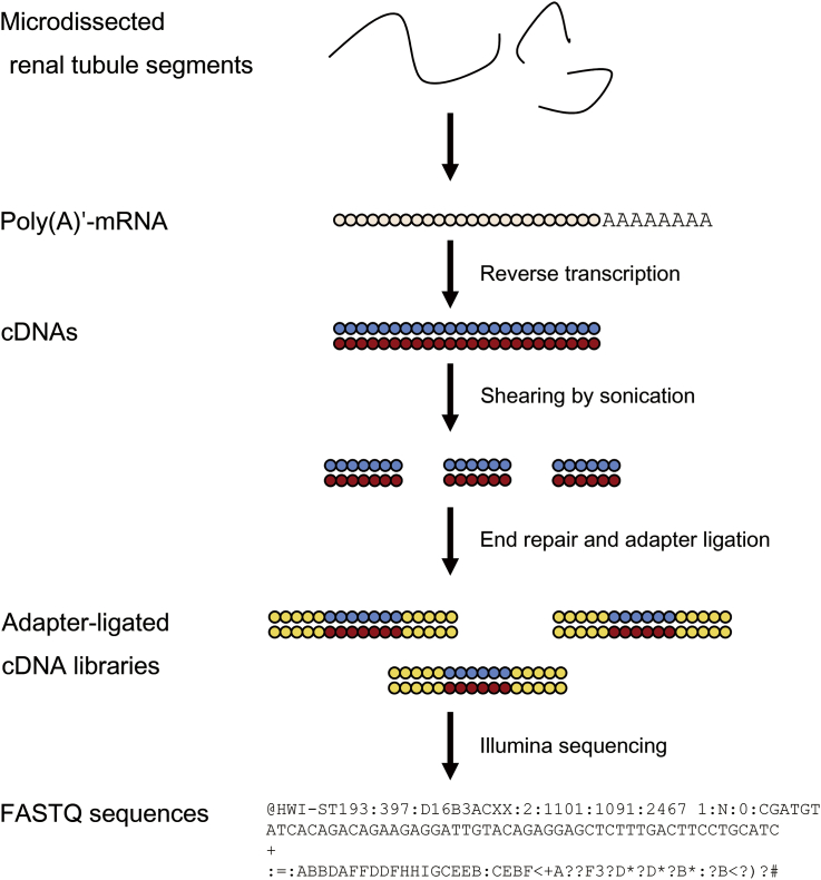
The overall workflow for the construction of cDNA libraries for RNA-seq of microdissected renal tubule segments is shown in Fig.┬Ā1. The microdissected renal tubule segments are lysed in mild cell lysis condition, and mRNAs are released from the cell lysate.
Cell lysis
An experienced dissector can collect 1ŌĆō4 mm (typically 500ŌĆō2,000 cells) of renal tubule segments within 2ŌĆō4 hours. Provided that a renal tubular epithelial cell contains Ōł╝1 pg of total RNAs, there are likely less than 1 ng of total RNAs in the collected sample. Because a conventional RNA-seq method that involves RNA fragmentation and reverse transcription with random hexamer primers (e.g., Illumina TruSeq protocol) requires a minimum of 100 ng of total RNAs as starting material, a highly sensitive method capable of creating cDNAs from a very small amount of total RNAs is needed for RNA-seq of renal tubule segments. For this work, the author used a modified version of the single-cell RNA-seq method that was originally developed for transcriptomic profiling of human oocytes [12].
To lyse the dissected tubules and release mRNAs, 20 ╬╝L of mild cell lysis buffer [0.9├Ś PCR Buffer II without MgCl2 (Life Technologies, Grand Island, NY, USA); 1.35┬Āmmol/L MgCl2 (Life Technologies); 0.45% Nonidet P-40 (Sigma-Aldrich, St. Louis, MO, USA); 4.5 mmol/L dithiothreitol (Life Technologies); 0.18 U/╬╝L┬ĀSUPERase-In (Ambion, Grand Island, NY, USA); 0.36 U/╬╝L┬ĀRNase inhibitor (Ambion); 12.5nM UP1 primer (5ŌĆ▓-ATATGGATCCGGCGCGCCGTCGACTTTTTTTTTTTTTTTTTTTTTTTT-3ŌĆ▓); dNTP mix (0.045┬Āmmol/L each); and nuclease-free water] is added to the PBS containing dissected tubules and mixed well using a pipette. This mixture is spun down at 7,500 g at 4┬░C for 30 seconds, heated at 70┬░C for 90 seconds to release mRNAs, and then spun down again at 7,500 g at 4┬░C for 30 seconds. Then, 0.5 ╬╝L of the cell lysate is taken and added to a new 0.5-╬╝L PCR tube containing 4 ╬╝L of the same cell lysis buffer to make a total of 4.5 ╬╝L. The last step minimizes the dilution of the reagents for reverse transcription by PBS. This cell lysate should be used immediately for the first-strand synthesis.
Alternatively, total RNAs can be isolated from microdissected tubule segments using silica membrane columns. When columns are used, RNAs should be eluted in as small volume (Ōł╝5 ╬╝L) as possible. An advantage of column-based RNA isolation over direct cell lysis is that RNAs can be stored in a ŌĆō70┬░C freezer for future work.
Reverse transcription and amplification
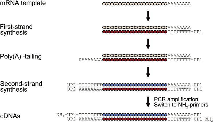
The method for cDNA synthesis used in the nephron RNA-seq is shown in Fig.┬Ā2. This homopolymer-tailing method uses a pair of universal oligo-dT primers and poly(A)ŌĆ▓-tailing of 5ŌĆ▓-ends to allow for PCR amplification. Despite several shortcomings such as limited coverage of proximal exons, bias toward 3ŌĆ▓-end, and loss of strand information, this method is sensitive enough to reliably amplify mRNAs from total RNAs as small as 20 pg [12]. The first-strand synthesis is started by adding 0.5 ╬╝L of reverse transcriptase mix [13.2 U/╬╝L┬ĀSuperScript III reverse transcriptase (Life Technologies); 0.4 U/╬╝L┬ĀRNase inhibitor (Ambion); and 0.07 U T4 gene 32 protein (Roche Diagnostics)] to 4.5 ╬╝L of the cell lysate to make 5 ╬╝L. If the total RNAs were isolated using silica membrane columns, 0.5ŌĆō1 ╬╝L of the total RNA is added to 4ŌĆō4.5 ╬╝L of the same cell lysis buffer (see the previous section) to make the total volume of 4.5 ╬╝L, and then 0.5 ╬╝L of the reverse transcriptase mix is added. Because the cell lysis step is not needed, NP-40 can be replaced with the same volume of nuclease-free water. The UP1 primers in the cell lysate capture poly(A)ŌĆ▓-mRNAs.
All the steps following the first-strand synthesis leading to cDNA amplification are identical to the previously published protocol [7], [12]. After removing excess primers, a poly(A)ŌĆ▓-tail is added to the 5ŌĆ▓-end of the DNAŌĆōRNA hybrid molecule (the product of the first-strand synthesis) by terminal transferase to allow for primer annealing in the next step, and the RNA template is removed by RNase H. Then, the second-strand synthesis is performed using a second universal primer (UP2, 5ŌĆ▓-ATATCTCGAGGGCGCGCCGGATCCTTTTTTTTTTTTTTTTTTTTTTTT-3ŌĆ▓) annealing to the poly-(A)ŌĆ▓ tail added to the 5ŌĆ▓-end in the previous step. Finally, this cDNA molecule is amplified (the first-round PCR, 18ŌĆō20 cycles) using the same universal primers (UP1 and UP2) and a high-performance DNA polymerase [TaKaRa Ex Taq HS DNA polymerase (Clontech Laboratories, Mountain View, CA, USA)].
Once the first-round PCR is complete, a quantitative real-time PCR (qRT-PCR) for a housekeeping gene (e.g., glutaraldehyde-3-dehydrogenase, beta-actin) is performed to see if the reverse transcription and amplification are successful. A successfully amplified sample will show an amplification curve that begins to rise before 20ŌĆō25 cycles of qRT-PCR. If the qRT-PCR is successful, the cDNAs amplified in the first-round PCR are further amplified (the second-round PCR, 9ŌĆō12 cycles) using NH2-modified universal primers [5ŌĆ▓-NH2-UP1, 5ŌĆ▓-(NH2)-ATATGGATCCGGCGCGCCGTCGACTTTTTTTTTTTTTTTTTTTTTTTT-3ŌĆ▓; and 5ŌĆ▓-NH2-UP2, 5ŌĆ▓-(NH2)-ATATCTCGAGGGCGCGCCGGATCCTTTTTTTTTTTTTTTTTTTTTTTT-3ŌĆ▓]. The purpose of this switch to NH2-modified primers is to minimize the amount of primer sequences appearing in the final cDNA libraries. The total number of PCR rounds should not exceed 32 because excessive amplification likely introduces more PCR errors.
Preparation of adapter-ligated cDNA libraries
To create adapter-ligated cDNAs compatible with Illumina sequencing, the cDNAs amplified in the previous step are sheared into Ōł╝200 bp fragments by sonication using a Covaris S2 system (Covaris Inc., Woburn, MA, USA)┬Āand then ligated to adapters. Before committing many samples to the adapter ligation process, the condition for sonication needs to be optimized so that the average size of the fragments is around 200 bp. After sonication, the cDNA fragments are cleaned up and eluted in 50 ╬╝L of nuclease-free water. The adapter ligation process is done on a Mondrian SP+ workstation (NuGen, San Carlos, CA, USA) using an Ovation Ultralow library prep system (NuGen). Finally, the adapter-ligated cDNAs are amplified with 10ŌĆō18 rounds of PCR and visualized on 2% agarose gel to select cDNAs within 200ŌĆō400 bp. The concentration of the final cDNA library is determined using a Qubit fluorometer (Invitrogen, Grand Island, NY, USA). A good cDNA library will give a concentration ranging from 1 to 5 ng/╬╝L.
Using adapters with multiplexed barcodes, cDNA libraries from multiple samples can be mixed into a single library for sequencing. The barcodes are 6-nucleotide-long DNA sequences incorporated in the stem or arm of the adapter molecule, and they can be used as identifiers for individual libraries. Each library is prepared using a barcoded adapter, and cDNA libraries with different barcodes are mixed in the same amount (e.g., 10 ng each) so that each library can be sequenced at the same depth. This multiplexing technique can save considerable amount of resource by enabling researchers to obtain sequences from multiple samples in a single sequencing run without significant loss of depth of sequencing. For example, 8 barcoded libraries can be mixed into 1 sample and sequenced to generate Ōł╝30 million sequences per each library. This depth of sequencing is usually good enough for differential expression analysis.
Next-generation sequencing
The technical details of Illumina sequencing are reviewed in the article by Metzker [9]. In the Nephron RNA-seq project [7], the adapter-ligated cDNA libraries were sequenced at the Genomics Core Facility of the National Heart, Lung, and Blood Institute using an Illumina HiSeq 2000 platform (Illumina Inc., San Diego, CA, USA) to generate 50-bp paired-end reads. Because it is usually not feasible for a small individual laboratory to own and operate an expensive sequencer, adapter-ligated cDNA libraries are usually sent to a core laboratory or a company that offers sequencing as a paid service. The choice between single-┬Āand paired-end sequencing depends on the purpose of the transcriptomic study to be conducted and resources available. Although paired-end sequencing enables more accurate mapping and thereby generates more information on the transcriptome, it takes longer and costs more money than single-end sequencing does. Paired-end sequencing is preferred for a deep profiling of transcriptome, whereas single-end sequencing usually suffices when the primary goal is differential expression analysis of known genes.
Analysis of RNA-seq data
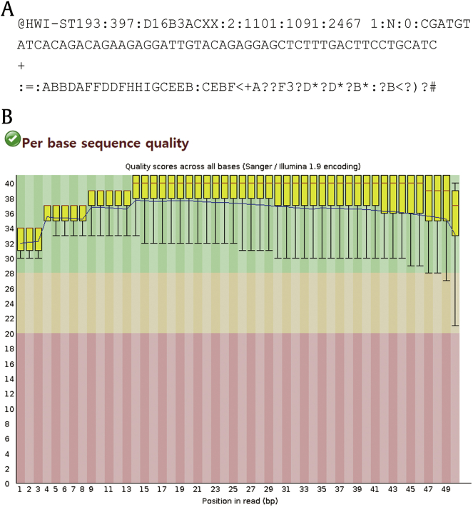
The nucleotide sequences of cDNA libraries are reported in FASTQ format, ŌĆ£FASTA with quality scores.ŌĆØ Fig.┬Ā3A is an example of a FASTQ sequence reported by an Illumina platform (Illumina Pipeline version 1.9). A FASTQ file normally uses 4 lines per sequence. The first line begins with a ŌĆ£@ŌĆØ character and bears information on machine ID, flowcell ID, coordinates on a flowcell, and a barcode sequence. The second line is the actual nucleotide sequence. Line 3 begins with a ŌĆ£+ŌĆØ character and is optionally followed by the same sequence identifier. Line 4 is ASCII representation of the quality scores for the sequence in the second line. In Illumina pipeline (since version 1.4), the quality score of a nucleotide (called Phred score) is determined by Q┬Ā= ŌĆō10┬Ā├Ś log10p, where p is the probability that the nucleotide is wrong, and converted to ASCII code by adding 33. For example, if the quality score for a nucleotide is 50, then the probability that the nucleotide is wrong is 10ŌĆō5. Its decimal ASCII code is 83, which is S.
Before the main analysis, the overall quality of these FASTQ reads needs to be assessed┬Ābecause inclusion of poor-quality nucleotides likely leads to erroneous mapping. Fig.┬Ā3B is a snapshot of a bar graph for quality scores at each nucleotide position. This graph was created using FastQC, a quality assessment tool available at http://www.bioinformatics.babraham.ac.uk/projects/fastqc/. Poor-quality nucleotides with a low-quality score need to be trimmed off to improve mapping quality. The author used a trimming program Trimmomatic [13] to inspect each sequence and trim off nucleotides with quality score lower than 30. If the remaining sequence is shorter than 35 nucleotides, the whole sequence was discarded. In addition to sequencing-quality scores, other measures of library quality such as overrepresented sequences, GŌĆōC content, sequence length distribution, or sequence duplication can also be analyzed using FastQC. A few red flags in this test do not necessarily mean that the library was poorly sequenced or prepared. Each red flag needs to be carefully inspected and judged on whether it is significant.
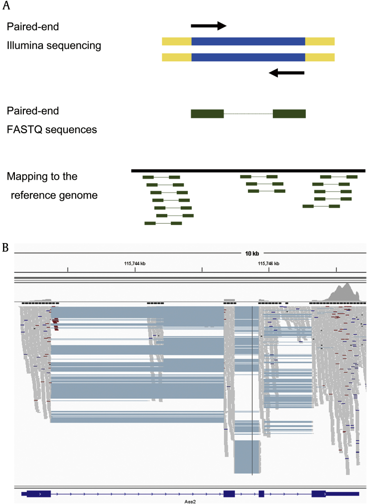
For transcriptomic analysis, the reported RNA-seq reads need to be mapped to the genome or transcriptome of a target organism (Fig.┬Ā4A). This mapping process is done using one of many programs dedicated to the analysis of RNA-seq reads. The author used STAR [14] to map RNA-seq reads to the rat reference genome (rn5). STAR is capable of precise mapping across exonŌĆōintron junctions and runs much faster than other mapping programs [e.g., Bowtie 2, TopHat2, and Burrows-Wheeler Aligner (BWA)]┬Ābut requires a large amount of computer resource (e.g., >16 GB of RAM and a multicore central processing unit). The mapped data are reported in a format called Sequence Alignment/Map or Binary Alignment/Map. These files are either further processed for downstream analysis or loaded onto a genome browser (Fig.┬Ā4B).
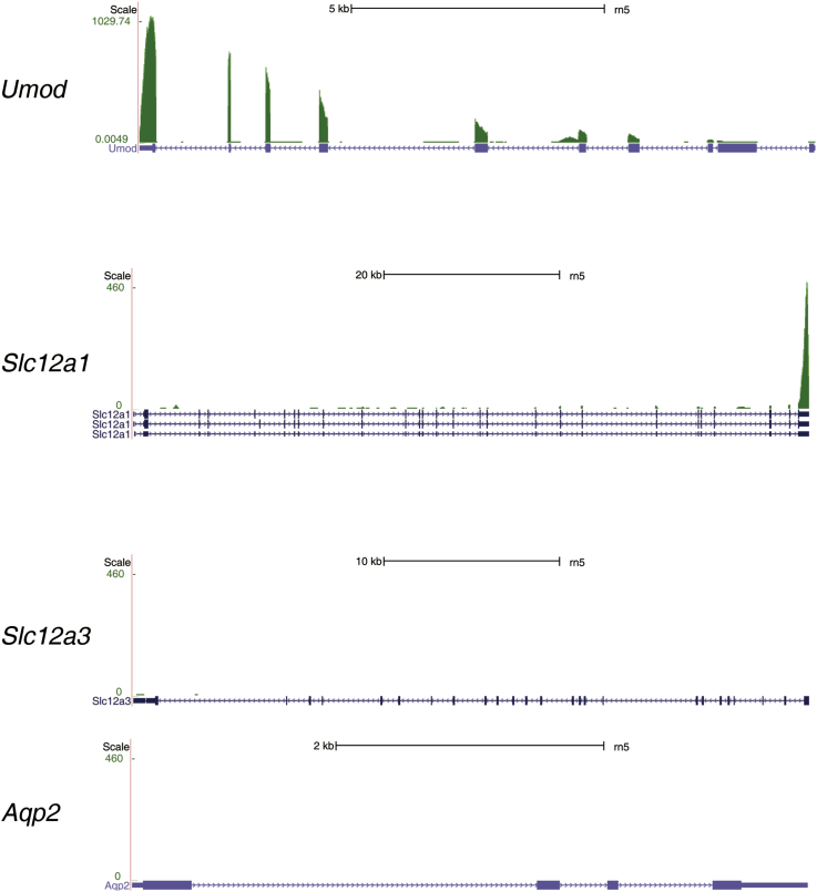
The mapped data need to be inspected in several ways to make sure that the overall library preparation and the mapping process were successful. First, the overall mapping rate, i.e., the proportion of reads mapped to the reference genome, should be higher than 70%. If this mapping rate is low, for example, <50%, it is mainly because the cDNA library did not contain sufficient amount of RNAs originating from the collected tubules, suggesting a failure in microdissection and/or cell lysis. In the nephron RNA-seq project, the author did not include samples that have the overall mapping rate lower than 65% [7]. Second, the annotated exons (i.e., protein-coding exons) should be enriched in the mapped data from a good cDNA library (e.g., >60% of reads mapped to annotated exons). If exons are not sufficiently enriched in an RNA-seq data set, contamination from genomic DNA or other sources should be suspected. A good RNA-seq data set may contain 10ŌĆō15% of reads mapping to introns┬Āas they likely originate from preprocessed mRNAs or retained introns. Third, as a sanity check, the mapped data should be visualized on a genome browser (Fig.┬Ā4B). By examining the expression of several markers or genes of interest on the genome browser, a researcher can judge whether the overall process of microdissection, sequencing, and mapping is successful. The expression of a tubule marker or a gene known to be expressed in the sample should be consistent with existing knowledge. For example, water channel aquaporin-2 (Aqp2, NM_012909) should be highly expressed in samples prepared from the connecting tubule and collecting ducts; aquaporin-1 in the proximal tubule and descending thin limbs; and the bumetanide-sensitive Na+ŌĆōK+ŌĆō2ClŌĆō cotransporter (Slc12a1, NM_001270617 and NM_001270618) in the thick ascending limb. In addition, markers of adjacent tubule segments should be minimally seen in the sample. Fig.┬Ā5 is a snapshot of an RNA-seq data set created from microdissected cortical thick ascending limb┬Āsegments, showing that uromodulin (Umod, NM_017082) and Slc12a1 are highly expressed, whereas the thiazide-sensitive Na+ŌĆōClŌĆō cotransporter (Slc12a3, NM_019345) and Aqp2 are not expressed at all.
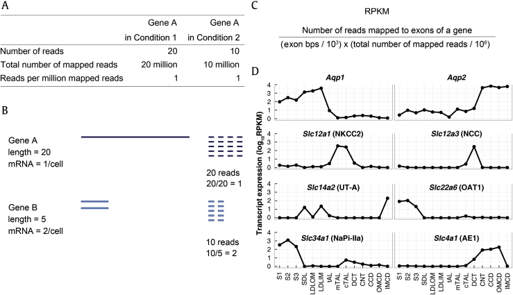
To measure gene expression in RNA-seq, the reads mapped to a transcript or gene are counted and summarized. This counting process requires a mapped file in the Sequence Alignment/Map or Binary Alignment/Map format and an annotation file for an organism. The annotation files are available at Ensembl (http://ensembl.org) or University of California at Santa Cruz (UCSC) database (http://genome.ucsc.edu) in the general feature format (GTF) or browser extensible data (BED) format. With these annotation databases, counting can be done using a tool such as htseq-count [15] or BEDTools [16]. Although the expression level of a gene is obviously proportional to the number of RNA-seq reads mapped to the gene, this number cannot be directly used to compare gene expression between 2 different genes or conditions without normalization. Figs.┬Ā6A, B illustrate the 2 most important factors that confound the read count data, namely the depth of sequencing (i.e., the total number of reads mapped to genome) and the length of a transcript (i.e., the number of nucleotides in exons of the transcript). To address these issues, a normalized measure called the read per kilobase exon model in million mapped reads (RPKM) was introduced to allow for comparison of gene expression across different genes and samples [17] (Fig.┬Ā6C). When the median RPKM values of tubule markers were obtained from replicates of 14 different renal tubule segments and plotted in line graphs, the axial distribution of tubule markers along the nephron was highly consistent with our prior knowledge of their distribution, demonstrating the precision of manual microdissection (Fig.┬Ā6D) [7].
When gene expression is compared between 2 conditions (e.g., control vs. treatment, normal vs. disease), a more robust statistical approach is used to model the raw count data into a statistical model for discrete data. Initial efforts to model RNA-seq data have been focused on the Poisson distribution [18]. Later, it was found that RNA-seq data have larger variability than that predicted by the Poisson distribution and that a model with increased variability (i.e., negative binomial distribution) is better at explaining RNA-seq data. For more information, readers are referred to articles and instruction manuals for individual software packages that normalize and analyze differential expression in RNA-seq using a negative binomial model (e.g., edgeR [19], DESeq [20], and DESeq2 [21]). As RNA-seq experiments begin to involve more replicates than were previously available and a more complicated experimental design begins to be applied, new analysis methods such as factor analysis [22] and surrogate variable analysis [23] are emerging.
Summary and future directions
This technical note introduced readers to RNA-seq of microdissected renal tubule segments, focusing on how to combine classical microdissection and a modified single-cell RNA-seq protocol. The data generated from this work are available both as supplemental data and a Web page (https://helixweb.nih.gov/ESBL/Database/NephronRNAseq/), allowing researchers to examine the expression of genes they are interested in. The raw FASTQ sequences obtained from 105 samples of glomeruli and renal tubule segments are available at Gene Expression Omnibus (GSE56743, http://www.ncbi.nlm.nih.gov/geo/query/acc.cgi?acc=GSE56743).
Although tubule-level transcriptome data will continue to generate new insights into the functions of the nephron, the transcriptomic research in nephrology will eventually advance to a single-cell level in the near future. Recent technical advances have made it possible for scientists to profile single-cell transcriptomes and reveal heterogeneous and stochastic nature of gene expression in individual cells [24], [25], [26]. Furthermore, single-cell RNA-seq has been used for marker-free decomposition of tissues into cell types, thereby allowing researchers to identify a new cell type without prior knowledge of cell markers [26], [27]. The author believes that these advances achieved in single-cell biology of other cells and organs can be reproduced in kidney research.
 PDF Links
 PubReader
 Full text via DOI
 Download Citation
 Print
Print


")